Curl operation on the vector fields is often necessary for the study of Electromagnetics to find the circulation of the given field along a certain path.
Definition of the Curl
It is a vector whose magnitude is the maximum circulation of the given field per unit area (tending to zero) and whose direction is normal to the area when it is oriented for maximum circulation.
In simple words, the curl can be considered analogues to the circulation or whirling of the given vector field around the unit area. More are the field lines circulating along the unit area around the point, more will be the magnitude of the curl.
The direction of the curl vector gives us an idea of the nature of rotation. It always follows the right-hand thumb rule where the thumb denotes the direction of curl vector and finger denotes the way of maximum circulation of the unit area.
The Curl – Explained in detail
The curl of a vector field is the mathematical operation whose answer gives us an idea about the circulation of that field at a given point. In other words, it indicates the rotational ability of the vector field at that particular point.
Technically, it is a vector whose magnitude is the maximum circulation of the given field per unit area (tending to zero) and whose direction is normal to the area when it is oriented for maximum circulation.
First of all, let me explain what do we mean by the circulation of the field. Let us consider any vector field is present in the region and let us also assume that a line XY is present in the field as shown in the figure below.
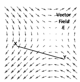
Now if we want to find the product of the component of the field along the line at every point and length of the line then we take line integral i.e.
In simple words, the line integration would give us the effect of the vector field along the given line.
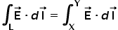
Now let us consider the same vector field. But now consider the small area say ‘ds‘ bounded by the closed path (L) is present within the field.
Now if I calculate the line integration of the given field along the path L, then in simple words, I would get the effect of the vector field along the L or boundary of the surface ‘ds‘. Now, what does this indicate? It is indicating how much the field is circulating the given area ‘ds‘. Isn’t it? It is represented as follows-

So this close line integration of the field around the boundary of the surface ‘ds’ is called as the circulation of the vector field. In layman’s words, it indicates the rotating or whirling capacity of the field if the surface is allowed to rotate. More is the circulation, more would be the answer of this integration.
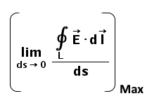
Now again jump to the definition of the curl. It requires maximum circulation per unit area i.e. area should approach to zero. So, mathematically it can be written as follows
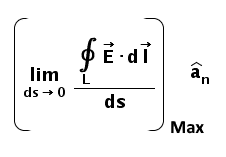
Now the final part of the definition that is the direction of the curl vector. According to the definition, it is normal to the area/surface such that the surface is aligned for the maximum possible circulation. Now, this can be easily determined using the right-hand thumb rule where thumb denoting the axis of the rotation if the surface is allowed to rotate according to the circulation of the field. And this will be the direction of the curl vector.
So mathematically, the definition would be as shown in the following figure where the bracketed term is the maximum circulation as discussed above and the unit vector according to the right-hand rule.
The Curl symbol and its representation
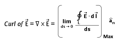
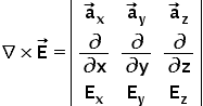
The curl of the vector field E is represented as ∇ × E. And finally, the representation of the curl of the vector field is given as-
The derivation of the Curl formula
Few Assumptions
The curl, in simple words, is the rotating or whirling nature of the vector field at a given point. Again in simpler words, it can be explained as – Assume that I have put a small surface at that point in the hypothetical vector field similar to force. Let us also assume that the surface has a fixed center but flexible axis. Then, this surface can rotate about the particular axis. The position of the axis and magnitude at that point for the maximum rotation can be considered as the Curl of this vector field.
As I have assumed the vector field is similar to force, it would be able to rotate that imaginary surface. But actually, for any other vector field, we would say the circulation of the field lines around that surface. Isn’t it? More circulation more curl. And as I explained in the last article, the numerator of the above formula denotes the circulation.
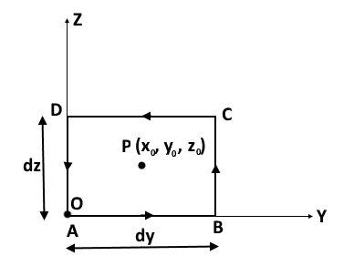
Assume that any vector field E is present in the region and we are finding the curl at any point within the field say P(x0, y0, z0).
Now according to the definition, the field lines of E will be circulating along the differential surface present at point P. And the axis of the curl will be decided using right-hand rule so that maximum circulation of the field is possible at that position. This position or orientation of the axis can be anywhere in the space. But for simplicity consider the axis along positive X-axis. Actually, the complete curl effect will be the combined effect (vector addition) of all three axes together i.e. along X, along Y and along Z.
As I am assuming the curl-axis along +X axis, I have to show the differential or small surface dS in YZ plane (bounded by ABCDA) and the circulation of the field in anticlockwise direction as shown in the figure below. This is according to the right-hand rule where thumb denoting the axis which is perpendicular to the surface and fingers denoting circulation of the field.

I am assuming the differential surface dS i.e. infinitesimally small surface bounded by differential lengths. Hence the line integration at the given point can be thought as the multiplication of the field value i.e. E and the differential length at that point.
The Intuitive derivation for the Curl formula
Let me again present the definition of the curl.
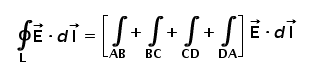
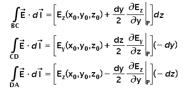
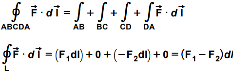
Let us calculate the close line integration in the numerator. As our small surface is bounded by four lengths viz. AB, BC, CD and DA. So this close line integration is calculated as –
Consider the very first integration i.e. from A to B. Let me present the diagram once again.
The length AB is the infinitesimally small length along Y-axis hence it can be considered as ‘dy’. The value of the function E at the location AB can be approximated using Taylor’s series.
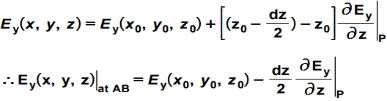
I have explained in previous article, how any function can be expanded around the given point in terms of spatial derivatives. In this case, the y-component of the field E can be expressed with Taylor’s series expansion around P(x0, y0, z0) as shown below. I am considering only y component of the vector field E i.e. Ey for a reason. Can you guess why?

I have considered only Ey because I am considering the integration from A to B. So for this integration, I need the component of the field E along AB i.e. along Y-axis, hence only Ey . Now the given line AB is at distance (dz/2) below from the point P. Hence from the above formula, we can consider only the term consisting derivative w.r.t. z. Also, z is taken equal to [z0 – (dz/2)]. So the value of Ey at the location of the line AB is as follows –
So the integration of E along AB can be written for the differential case as follows. The Ey is given by the above equation and the dl is dy as stated initially.
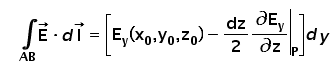
You can easily work out in a similar manner to get the remaining integrals for BC, CD and DA. In each case, the value of the field E and dl are modified accordingly.
So for the complete close integration along ABCD i.e. circulation of the field, we need to add all these four terms together and we will get the following.
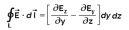
But, wait. Can you observe the term dydz. What does this represent? It is the area of the differential surface dS that we have assumed at the starting of our discussion. Isn’t it? Also as we have assumed this area to be very small, differentially small we can say it is approaching zero. So above relation can be written as follows
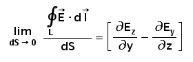
Bingo! Check out the left-hand side of the above equation. It is exactly the same as the definition of the Curl. Am I right? So this is the expression of the curl of our assumed vector field E having axis along X-axis (as we have assumed so initially).
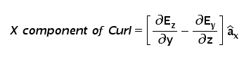
On similar lines, we can proceed step by step as we did here and find the Y and Z components of the Curl.
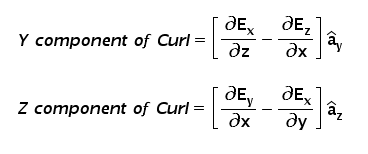
Rather than these three formulas for different components, the complete Curl formula in matrix form is represented as follows. This matrix form formula after simplification would also lead to the above three formulas.
Curl Formula in different Coordinate Systems
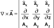
Curl Formula in Cartesian Coordinate System
Let the vector field is A whose curl operation is to be calculated. Then A would have the standard form as follows – \overrightarrow A=A_x{\widehat a}_x+A_y{\widehat a}_y+A_z{\widehat a}_z. Then curl is defined as follows
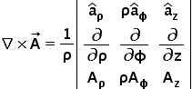
Curl Formula in Cylindrical Coordinate System
If A is the vector field whose curl operation is to be calculated, then for cylindrical coordinates, it would have the standard form as follows – \overrightarrow A=A_\rho\widehat a\rho+A\phi{\widehat a}_\phi+A_z{\widehat a}_z Then curl is defined as follows: –
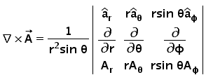
Curl Formula in Spherical Coordinate System
For spherical coordinates, A would have the standard form as follows – \overrightarrow A=A_r{\widehat a}_r+A_\theta{\widehat a}_\theta+A_\phi{\widehat a}_\phi Then curl is defined as follows: –
Curl of a Vector field explained with an intuitive example.
Few Assumptions for the Curl Example
Let us consider the surface of the imaginary water current. It is the best example of the vector field.
After all, a vector field can be considered as the set of vectors present in the space defined by a certain function. In other words, each point in the field bears a vector whose magnitude and direction is decided by the given function. And the surface of the water current can be easily simulated as a vector field.
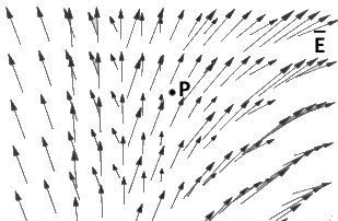
The velocities of the water current at different points of the surface form the set of vectors i.e. field as shown in the following figure. The magnitude and the directions of these individual vectors are governed by a certain function.
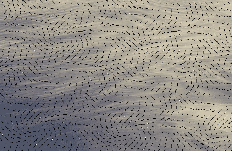
Again for simplicity, we can assume that the velocity vector is nothing but the force that is experienced by any point object placed at that point. So the above diagram of the velocity vector field becomes the force vector field. This way we can say that these force vectors are responsible for any movement of the object that is placed on the surface.
Now let us assume that a small piece of paper or lamina of area ‘ds’ is put on this water surface. For simplicity let us consider the ‘ds’ to be a square. Also, consider that this ‘ds’ is a hypothetical area which doesn’t flow along with the stream of water but remains stationary at the given point. Yes, but assume that it can rotate about its axis.
Case 1: Uniform stream flow
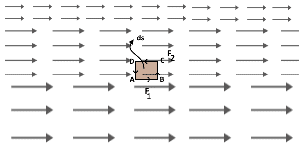
Consider the water stream which having uniform current all the way. Pictorially it can be shown as below where each force vector in the field is of equal magnitude with the same direction.
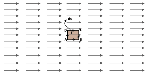
Now let me explain this by another way i.e. using the concepts of line integration. We know that the line integration of the vector field along any path is the sum of all the infinitesimal products consisting of the field value (parallel to the path) and the infinitesimal length.
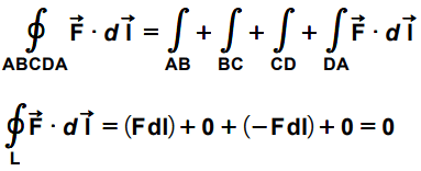
The assumed surface ‘ds’ is bounded by the closed loop ABCDA. Now let us find the line integration of the field F along this path ABCDA i.e. along the boundary of the ‘ds’. As we have assumed our area to be infinitesimal, all the lengths i.e. AB, BC, CD and DA will be infinitesimal. So the line integration of the field along any of these infinitesimal lengths will be just the product of the field along the path and infinitesimal length (dl).
Note the TWO points in above integration. First, the line integrations along BC and DA are both zero. The reason is that the angle between F and dl are 900 and 2700 respectively. And for the line integration, we want the component of the field along (parallel to) the path i.e. Fcosθ. So they both are zero.
Second, the integration for CD is negative. The reason for this is also the same, the angle θ. Here it is 1800. Both F and dl are going anti-parallel.
Now the line integration along the ABCDA can be called as the circulation of the field lines for the surface ‘ds’. In other words, this circulation i.e. the answer of this integration is responsible for the net circulation of the area ‘ds’.
In our case, this is a zero. So the rotational nature is zero i.e. the curl of the field is zero.
Case 2: Stream flow intense downside
Consider the same stream flow. But in this case, assume that the function of the field is such a kind where the force vectors are strong at the downside and weak in the upside.
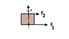
In this case, as you can see from the figure, the force on the ‘ds’ is not uniform. It is higher in the downside while lower in the upside. So this unbalanced force on the ‘ds’ would act as a rotational force and the ‘ds’ would rotate as shown in the figure below. The surface also can translate in the water current but we have assumed that it is fixed at a point and allowed only to rotate.
Mathematically, we can say that the net circulation of the field is not zero. And this is responsible for the circulation of the ‘ds’.
Case 3: Stream flow intense upside
This would be similar to Case 2. In this case, also, the net circulation of the field is not zero and responsible for the circulation of the ds.
But one very important thing we can notice here that the nature of the rotation. In case 2 the nature of rotation was anticlockwise as F1 is greater than F2. But in this case, it will be clockwise. If we consider the axis of rotation according to the right-hand rule then the thumb direction is opposite in both of the cases.
Takeaway from the Curl Example
We have modelled a vector field as a surface of the water current. This may not be 100% true as the actual field may occupy the 3D space.
So in case of the actual vector field, this Curl example should be stretched further to get the axis of the rotation of ‘ds’ such that maximum circulation is possible.
So curl of a vector field is the rotating or whirling nature of the field at the point of interest. More are the lines of the field whirling around the point, more will be the curl.
Do not forget to check our Awesome GATE courses.