Gradient calculus is frequently used in Electromagnetic Theory. Particularly, it is significant while understanding the relation between Electric Field and Potential. This article discusses the details of the Gradient in Electromagnetics.
A formal definition of the Gradient
The Gradient of the scalar function/field is a vector representing both the magnitude and direction of the maximum space rate (derivative w.r.t. spatial coordinates) of increase of that function/field.
The Gradient in simple words
Regardless of the fancy definition above, you can assume the “Gradient” as the other name for the “Differentiation”.
In a single variable function, say y = f(x), the derivative (dy/dx) represents the rate of change of ‘y‘ with respect to ‘x‘. In other words how much is the change in ‘y‘ (dy) for a change in ‘x‘ (dx). It represents the slope of the tangent at that point.
In multivariable function, the value of the function may change with respect to any variable, because of change in one or two or all. So it can have three different derivatives for each coordinate. The combined effect with a direction may be considered as the Gradient.
The Gradient – Explained in detail
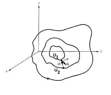
For simplicity consider the Cartesian coordinate scalar function U (x, y, z).
U = constant would represent the certain, surface/contour as shown in the figure for U = U1, U = U2, U = U3.
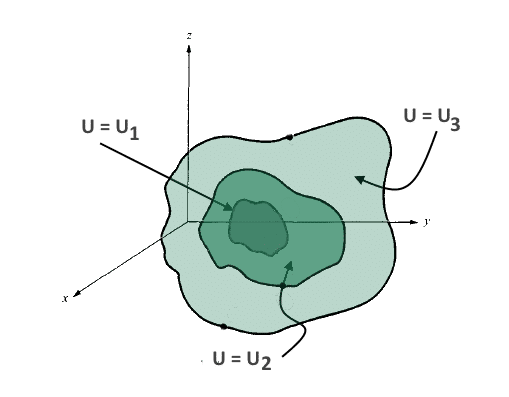
The small change in this function i.e. dU can be because of the change in x or y or z or all. The change can be thought as the surface U1 tries to occupy U2 so the change is U2 – U1 and likewise.
The change [dU]x because of change in x can be represented as- (∂U/∂x)dx. This is according to the elementary definition of the derivative. As we want the change in U introduced because of change in x, firstly we need the rate of change of U w.r.t. x i.e. (∂U/∂x) then multiplied by the small change dx. The derivative used here is the partial derivative because the function U is also the function of other variables and when we consider the change in it because of x, we inherently assuming that other variable i.e. y and z to be constants.
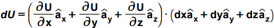
On a similar line, we can write the [dU]y and [dU]z and finally the change in U i.e. dU can be represented as
dU= (∂U/∂x)dx + (∂U/∂y)dy + (∂U/∂z)dz
Let us slightly modify the above equation as –
Aren’t previous equation and this equation same? 100% same. Try the dot product above and you will end up with the former equation. We have modified the equation for a reason, you come to know.
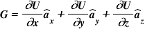
Let us call the first bracketed term as G and the term in the second bracket, as you already know in the topic of line integration, is dl. So dU can be written as,
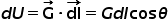
So, we can write as,

Carefully examine the term what we called ‘G‘

Can you guess, what does this term represent?
This G is representing the rate of change of function U w.r.t. spatial coordinates x, y and z i.e. the space rate. (Have you recalled this word from the definition?)
One more thing you can easily notice that G is indicating the rate of change of the complete function comprising the x-component i.e. change along x, y-component i.e. change along y and z-component i.e. the change along z. So overall, with vector representation, it is giving us the magnitude as well the direction for the rate of change of U w.r.t. x, y and z. Summarizing G is denoting the magnitude and direction of the space rate of increase of the scalar function U.
Note that, I have used the word “Rate of increase in U”. Can you guess why have I done so? The G is giving us the rate of change of function U, that’s fine. We discussed this well up to this point. But it can be the rate of increase or maybe the rate decrease. Then why I am saying only the rate of increase.
This can be understood as – with the incremental increase in the spatial variables (dx, dy, dz which are taken positive only) if the final value of U is higher than the initial value then the vector direction is towards final value with positive unit vectors. But if its final value is less than the initial value then the direction would be reversed because of the negative sign appearing with the unit vectors. Why negative sign? Apply the simple rule, change equals final minus initial. In other words, this direction is also pointing the higher value.
So summarizing over the complete 3D space, the direction of G would always be pointing towards the higher value of the scalar function U. So we can say that G is denoting the magnitude and direction of the space rate of increase of the scalar function U.
Why am I talking so much about this G?
Because recall the definition for gradient – The Gradient of the scalar function/field is a vector representing both the magnitude and direction of the maximum space rate (derivative w.r.t. spatial coordinates) of increase of that function/field.
From the definition, we can say, the term G is satisfying all the conditions to be called the Gradient operator. Hence the gradient of the scalar field U is given by –
One point is worth noting here that according to the definition, the Gradient is the maximumspace rate of the function. Once again have the look at the equation-

dU/dl is the space rate i.e. rate of change of U w.r.t. x, y and z. And for this to be maximum, it would be along the G so θ = 0 as shown in the diagram below.
So we can define the Gradient as,

The Gradient Symbol
The gradient of the scalar field U is denoted as ∇ U.
The direction of a Gradient Vector
So we have discussed the definition for the Gradient. In one sentence, it is magnitude and direction of maximum space rate of a scalar function. Now, can you draw this Gradient vector (G or ∇ U) indicating proper direction?
The direction of the Gradient Vector must be perpendicular or normal to the given scalar field/function. Refer to the diagram just above, the direction of G is normal to the U1. Can you drop the comments, why so?
How to represent the Gradient in different Coordinate Systems?
Let the scalar function or field is ψ. Assume that we are required to apply the gradient operation on this ψ. This would be represented as-
∇ ψ
The following points are worth noting while applying the gradient operator: –
- The answer would be a vector quantity.
- There must not be (•) or (×) between the ∇ and ψ.
Let V be the scalar field whose gradient to be calculated,
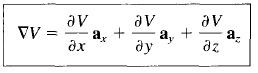
Gradient Operation in Cartesian Coordinates
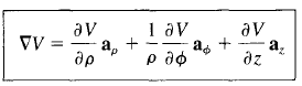
Gradient Operation in Cylindrical Coordinates
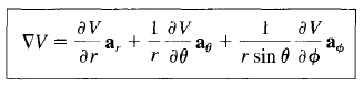
Gradient Operation in Spherical Coordinates
Gradient explained with a simple intuitive example!
Consider a hypothetical room whose temperature is different at every point and depends on the coordinates of the point. In other words, the temperature at each point inside the room is a function of (x, y, z) coordinates.
We know that temperature is a scalar quantity and it is a function of spatial coordinates. So we can say, the room assumed above is an example of the scalar function or scalar field.
Now, let us assume that this room is like an oven for us and we put a cookie anywhere inside it. But we want to bake the cookie as quickly as possible. Let us also assume that, this imaginary room cum oven posses some magical power by which the object inside it, can float anywhere within the room. In other words, the object can adjust its own position in the space according to the command/ program fed by you.
Is the scene ready in your mind? Now you are a programmer and you are supposed to write a program (of course the simple one) so that the cookie can be baked as quickly as possible, say within the minimum time.
What would you do? Can you think of the flowchart for the required program? What could be your first step? Our aim is to bake the cookie as quickly as possible. How can this be achieved? Any guess?
Of course, this can be achieved by constantly moving the cookie towards the point of higher temperature (than previous) and make it to the point of highest temperature. So our program must always point the cookie towards the neighbourhood point which has a higher temperature than previous. So what our program shoul do? It would check all the direction i.e. x, y and z to find where the change of temperature is maximum. How? Of course, by the derivative. You know the derivative gives us the rate of change of function; in this case, the derivative with respect to x, y and z i.e. spatial coordinates.
Now let us add the corresponding unit vectors with the derivative terms i.e. ax with X-direction derivative, ay with Y-direction derivative and az with Z-direction. So the combined vector formed is as shown below where T is the temperature inside the room at any point (x, y, z) i.e. the scalar function.
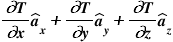
As a whole, this vector will always give the magnitude and the direction of the maximum rate of increase of the temperature inside the room. Can you notice that the vector above is nothing but a Gradient Vector! Isn’t it?
So the program of our Gradient example should actually be finding the Gradient of the scalar field (Temperature inside) and eventually to reach the maximum temperature point.
It should be noted that many facets of the above Gradient Example can be considered for this hypothetical program. Can you comment few?
Fundamental Properties of the Gradient of a Scalar Field
The Gradient is like the Derivative
The Gradient can be said as the similar operation of multi-variable differentiation in normal calculus but not exactly the same. In normal calculus the derivative gives us the rate of change of one function with respect to certain variable. It is giving information about the slope of the curve. But the Gradient is the special kind bundle of derivatives with respect to space coordinates (like x, y, z) with unified direction.
The Gradient operation operates on Scalar and gives back Vector
The answer of Gradient operation is a vector. It is evident from the Gradient Operator that each derivative term is associated with the respective unit vector.
The Gradient vector points towards the maximum space rate change
The magnitude and direction of the Gradient is the maximum rate of change the scalar field with respect to position i.e. spatial coordinates.
Let me make you understand this with a simple example. Consider the simple scalar function, V = x2 + y2 + z2. We know that this function, V = constant would give us the sphere. Let us consider the two values of the function V1 = 4 and V2 = 8. Now we can see that the function V is changing w.r.t. spatial coordinates i.e. x, y and z. The Gradient of the function at a point can be intuitively shown as below.
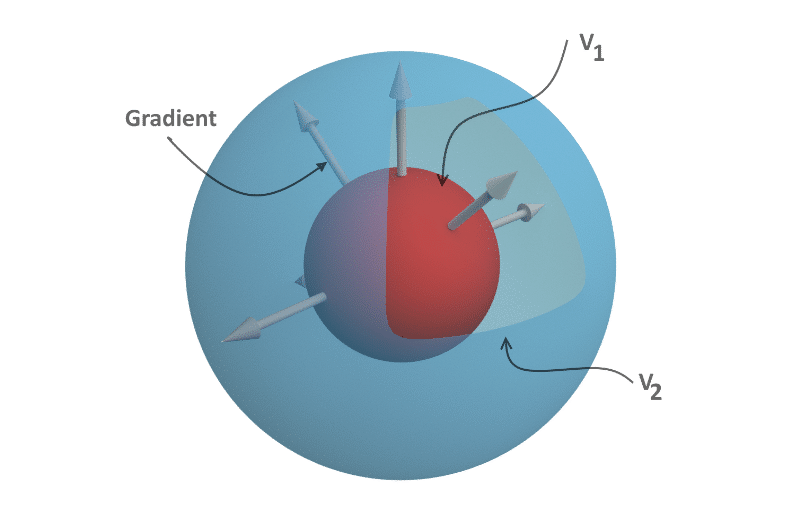
Gradient Vector is normal to the constant V Surface
The Gradient vector at any point is perpendicular to the constant V surface that is passing through that point. It could be probably the most useful for Electrostatics, amongst all the Gradient Properties. As seen from the above diagram, V1 and V2 are the V equal to constant surfaces. We can also assume intuitively that the function is gradually changing from 4 to 8. Hypothetically saying, if I am leaving from V1 to reach for V2 then I have to follow the perpendicular path between these surface to reach quickly. Isn’t it? In technical language, this is so because the change in the function is highest along the normal and hence the Gradient direction.
Do not forget to check our Awesome GATE courses.