LTI Systems Set-1

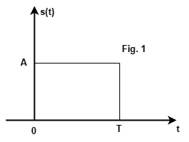
[1987 : 8 M] A rectangular pulse existing between t = 0 and t = T and having an amplitude A is to be received by a matched filter.

(a) Draw the impulse response of the matched filter labeling all important points and the axes.

(b) Find the signal shape at the filter output. Label all important points and the axes.

Ans: A rectangular response of the matched filter, is having an amplitude A is shown in Fig. 1.

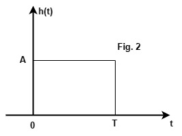
(a) The impulse response of the matched filter, is given by h(t) = s(-t+T)………(1)

where T is the duration of the pulse in Fig.1.

h(t) is shown in Fig.2

Note that for the given s(t)

h(t) is same as s(t).

(b) Filter output y(t) = s(t) * h(t)………..(2)

= s(t) * s(t)

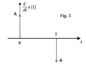
\int\limits_{t=-\infty}^t\left[s\left(t\right)\ast s_1\left(t\right)\right]dt………(3)

where s_1t=\frac{d\;s\left(t\right)}{dt} is shown in Fig. 3.

s_1\left(t\right)=A\delta\left(t\right)-A\delta\left(t-T\right)

\therefore y\left(t\right)=\int\limits_{-\infty}^ty_1\left(t\right)dt………..(4)

where

y_1\left(t\right)=s\left(t\right)\ast s_1\left(t\right)=\left[s\left(t\right)\ast A\delta\left(t\right)\right]-\left[s\left(t\right)\ast A\delta\left(t-T\right)\right]

Use the property of convolution with impulses:

s\left(t\right)\ast\delta\left(t\right)=s\left(t\right) s\left(t\right)\ast\delta\left(t-T\right)=s\left(t-T\right)

\therefore y_1\left(t\right)=As\left(t\right)-As\left(t-T\right)……..(5)

y₁(t) is show in Fig. 4.

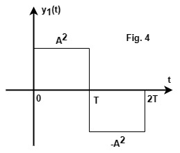
From (4), y₁(t) is integrated to get y(t)

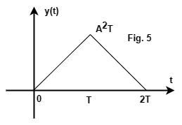
Values of y(t) are easily calcuated

from Fig.4, by seeing the accumulated area.

y(t) is shown in Fig.5

---

[1988 : 2 M] The transfer function of a zero-order hold is

(a) \frac{1-exp(-Ts)}s

(b) 1/s

(c) 1

(d) 1/[1-exp(-Ts)]

Ans: (a)

Explanation

Impulse response of zero-order hold is shown in Fig.1.

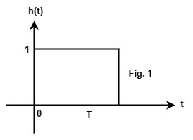
h(t) = u(t) – u(t-T)

∴ Transfer function, H(s) = Laplace transform of h(t)

= (1 – e^-Ts)/s

as u(t) ⟶ 1/s and u(t-T) ⟶ e^-Ts/s, from Time shifting property

---

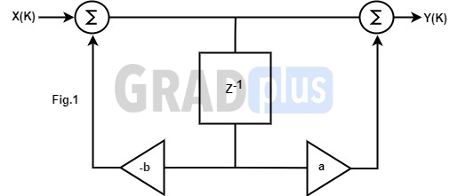
[1988 : 2 M] Consider a system shown in the Fig. 1 below. The transfer function Y(z)/X(z) of the system is

(a) \frac{1+az^{-1}}{1+bz^{-1}}

(b) \frac{1+bz^{-1}}{1+az^{-1}}

(c) \frac{1+az^{-1}}{1-bz^{-1}}

(d) \frac{1-bz^{-1}}{1+az^{-1}}

Ans: (a)

Let

x\left(k\right)\xrightarrow{ZT}X\left(z\right), y(k) ⟶ Y(z)

The system block diagram is redrawn in Fig. 2 to write the following relations:

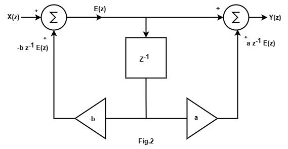
E(z) = X(z) – bz^-1 E(z), Y(z) = E(z) + az^-1 E(z)

or E\left(z\right)=\frac1{\left(1+bz^{-1}\right)}X\left(z\right) or

Y(z) = (1+az^-1)E(z)

Y\left(z\right)=\left(1+az^{-1}\right)\frac1{\left(1+bz^{-1}\right)}X\left(z\right),

\therefore Transfer\;function=\frac{Y\left(z\right)}{X\left(z\right)}=\frac{1+az^{-1}}{1+bz^{-1}}

The answer can also be obtained probably quickly by using Mason’s gain formula

Gains of the two existing Forward paths : M₁ = 1 and M₂ = a z^-1

Gain of the (only one existing) individual loop = -b z^-1

∆ = 1 – ∑ Individual loop gains = 1 + b z^-1

and ∆ ₁ = 1, ∆ ₂ = 1

\therefore\frac{Y\left(z\right)}{X\left(z\right)}=M=\frac{M_1\triangle_1+M_2\triangle_2}\triangle=\frac{1+az^{-1}}{1+bz^{-1}}

---

[1988 : 4 M] The output of a system is given in difference equation form as

y(k) = a y(k-1) + x(k)

where x(k) is the input. If x(k) = 0 for k ≠ 0, x(0) = 1, and y(0) = 0, find y(k) for all k. Determine the range of ‘a’ for which y(k) is bounded.

Ans:

The output y(k) of the system is given by

y(k) = a y(k-1) + x(k), y(0) =0

where the input x(k) is defined by

\left.\begin{array}{cc}\begin{array}{c}x(k)=0\\x(0)=1\end{array}&k\neq0\end{array}\right\}

∴ x(k) is a discrete impulse (or unit sample sequence)

x(k) = δ(k)

The impulse response, h(k) of the system is asked in this question, subject to the initial condition y(0) = 0

y(k) = a y(k-1) + δ(k)

Put the values of k:

\left.\begin{array}{cc}k=1&y(1)=a\;y(0)+\delta(1)=0\\k=2&y(2)=a\;y(1)+\delta(2)=0\end{array}\right\}

y(0) = a y(-1) + δ(0) = a y(-1) + 1

0 = a y(-1) + 1, y\left(-1\right)=-\frac1a=-a^{-1}

y(-1) = a y(-2) + δ(-1)

-\frac1a=a\;y\left(-2\right)+0, y\left(-2\right)=-\frac1{a^2}=-a^{-2}

etc

y(k) = -a^k, for k ≤ -1

y\left(k\right)=\left\{……,-\frac1{a^3},-\frac1{a^2},-\frac1a\;0\;0\;0\;……\right\}

For a = 1 =\left\{……,-1,\;-1\;-1,\;0\;0\;0\;……\right\}………(1)

\underset{Let\;a=2}{For\;a>1}=\left\{……,-\frac18,-\frac14,-\frac12,\;0\;0\;0\;……\right\}……….(2)

\underset{Let\;a=1/2}{For\;a<1}=\left\{……,-8,-4,-2,\;0\;0\;0\;……\right\}………(3)

As can be seen from (2), y(k) is bounded for |a| > 1.

---

[1989 : 8 M] For the input signal, x(t), shown in Fig.1:

(a) Sketch the impulse response, h(t), of the matched filter.

(b) Sketch the output, y(t), of the mathced filter. Fully label your diagram.

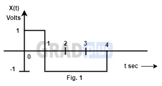
Ans:

(a) Impulse response of the matched filter in terms of its input x(t) is given by

h(t) = x(-t + T)………(1)

where T is the duration of x(t), T = 4

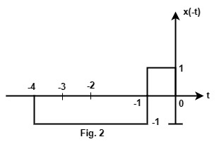
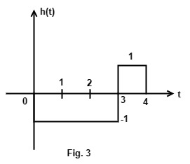
For the given x(t), x(-t) and

h(t) = x[-(t – T)]are shown in Fig. 2 & 3.

(b) Output of the matched filter

y(t) = x(t) * h(t) ………..(2)

Using the properties of convolution

y(t) can be easily evaluated by the following integral

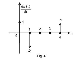
y\left(t\right)=\int\limits_{t=-\infty}^t\left[\frac{dx\left(t\right)}{dt}\ast h\left(t\right)\right]dt……..(3)

\frac{dx\left(t\right)}{dt} is shown in Fig. 4.

y\left(t\right)=\int\limits_{-\infty}^ty_1\left(t\right)dt ………………(4)

where y_1\left(t\right)=\frac{dx\left(t\right)}{dt}\ast h\left(t\right)=\left[1\delta\left(t\right)\ast h\left(t\right)\right]-\left[2\delta\left(t-1\right)\ast h\left(t\right)\right]+\left[1\delta\left(t-4\right)\ast h\left(t\right)\right]

y₁(t) = h(t) – 2h(t-1) +1h(t-4)………….(5)

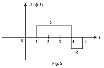
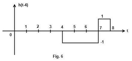
-2 h(t-1) and 1 h(t-4) are shown in Fig. 5 & 6.

y₁(t) = Fig. 3 + Fig. 5 + Fig. 6

y₁(t) is shown in Fig. 7

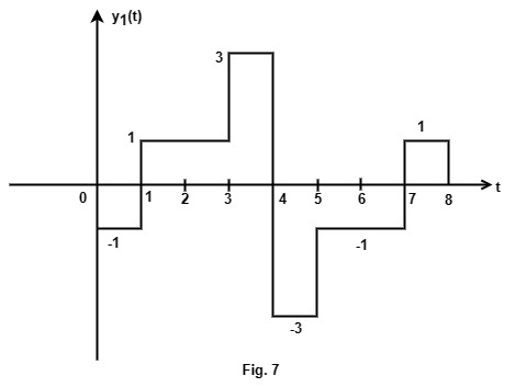
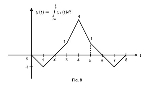
From (4), the output of the matched filter, y(t) is obtained as integration of y₁ (t).

Typical values of y(t) are calculated using the accumulated areas in Fig. 7.

y(t) is sketched in Fig.8.

---

[1990 : 2 M] The response of an initially relaxed linear constant parameter network to a unit impulse applied at t = 0 is 4e^-2tu(t). The response of this network to a unit step function will be

(a) 2[1-e^-2t] u(t)

(b) 4[e^-t-e^-2t] u(t)

(c) sin 2t

(d) (1-4e^-4t) u(t)

Ans: (a)

The given network is a LTI system. The impulse response is given as

h(t) = 4 e^-2t u(t)

i.e, the response to δ(t) is h(t).

For LTI system, if the input is integrated the output is also integrated.

As u\left(t\right)=\int\limits_{t=-\infty}^t\delta\left(t\right)dt

The response of the system to unit step function is given by

s\left(t\right)=\int\limits_{t=-\infty}^th\left(t\right)dt=\int\limits_{t=0}^t4e^{-2t}dt=\frac4{-2}\left[e^{-2t}\right]_0^t=2\left(1-e^{-2t}\right),\;t\geq0

= 0, t < 0

\therefore s\left(t\right)=2\left[1-e^{-2t}\right]u\left(t\right)

---

[1990 : 2 M] The impulse response and the excitation function of a linear time invariant causal system are shown in Fig. a and b respectively. The output of the system at t = 2 sec. is equal to

(a) 0

(b) 1/2

(c) 3/2

(d) 1

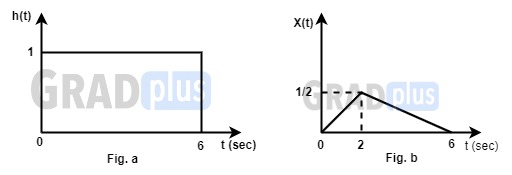
Ans: (b)

An LTI system is causal, if its impulse response, h(t) is zero for t < 0.

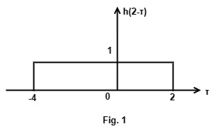
For the given causal L.T.I. system the output is given by

y\left(t\right)=x\left(t\right)\ast h\left(t\right)=\int\limits_{t=-\infty}^\infty x\left(\tau\right)h\left(t-\tau\right)d\tau=\int\limits_{t=0}^tx\left(\tau\right)h\left(t-\tau\right)d\tau

as x(t) = 0, t < 0 and h(t) = 0, t < 0

\therefore y\left(2\right)=\int\limits_{t=0}^2x\left(\tau\right)h\left(2-\tau\right)d\tau

For the given h(t) and x(t), h(2 – τ) and x(τ) are shown in Fig. 1 & 2.

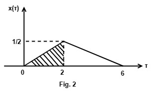
y(2) = Shaded area of the triangle shown in Fig. 2 = 0.5

---

[1991 : 2 M] An excitation is applied to a system at t = T and its response is zero for -∞ < t < T. Such a system is a

(a) non-causal system

(b) stable system

(c) causal system

(d) unstable system

Ans: (c)

Explanation

For the given system the response is zero prior to the application of the excitation. Such a system is called causal system.

---

[1991 : 2 M] The voltage across an impedance in a network is V(s) = Z(s) I(s), where V(s), Z(s) and I(s) are the Laplace Tranforms of the corresponding time functions v(t), z(t) and i(t). The voltage v(t) is

(a) v(t) = z(t). i(t)

(b) v\left(t\right)=\int\limits_0^ti\left(\tau\right)z\left(t-\tau\right)d\tau

(c) v\left(t\right)=\int\limits_0^ti\left(\tau\right)z\left(t+\tau\right)d\tau

(d) V(t) = z(t)+i(t)

Ans: (b)

Explanation

V(s) = Z (s) I(s)

Use property of FT pairs: Multiplication of two functions of s is equivalent to the convolution of the corresponding functions of time.

v(t) = z(t) * i(t)

According to the definition of convolution of two time functions, z(t) and i(t),

v\left(t\right)=\int\limits_{\tau=0}^ti\left(\tau\right)z\left(t-\tau\right)d\tau=\int\limits_{\tau=0}^ti\left(t-\tau\right)z\left(\tau\right)d\tau

---

[1992 : 2 M] A linear discrete-time system has the characteristic equation, Z³ – 0.81 z = 0. The system

(a) is stable

(b) is marginally stable

(c) is unstable

(d) stability cannot be assessed from the given information.

Ans: (a)

The roots of the characteristics equation are the poles. For discrete time system the poles should lie inside the unit circle in the z – plane for stability. In this problem the poles are given by z³ – 0.81 z = 0

z(z – 0.9) (z + 0.9) = 0

p₁ = 0, p₂ = 0.9, p₃ = -0.9. As all the three poles are inside the unit circle, the system is stable.